In my last blog post, which was about a million years ago, I described the generative nature of LDA and left the interferential step open. In this blog post, I will explain one method to calculate estimations of the topic distribution $\theta$ and the term distribution $\phi$. This approach, first formulated by Griffiths and Steyvers (2004) in the context of LDA, is to use Gibbs sampling, a common algorithm within the Markov Chain Monte Carlo (MCMC) family of sampling algorithms. Before applying Gibbs sampling directly to LDA, I will first give a short introduction to Gibbs sampling more generally.

Gibbs Sampling¶

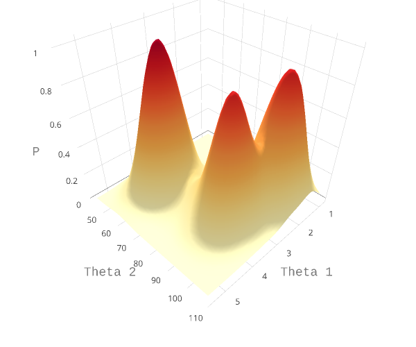
Gibbs sampling is useful when it is difficult (or impossible) to draw samples from a joint distribution of multiple variables, but easy to draw samples from conditional distributions. Let us assume our model has two parameters, $\theta_1$ and $\theta_2$. Under Bayesian inference, the parameter space for the variables is the joint distribution of the parameters, $P(\theta_1, \theta_2 ~|~ D)$, where $D$ is the data provided. This joint distribution can take any form. One artificial complex example is shown in Figure 1 below. When the number of parameters increase, this joint distribution becomes more and more complex, and is often impossible to solve analytically. The approach taken in Gibbs sampling is instead to sample from the conditional probability distributions $P(\theta_i~|~{\theta{j\ne i}},D)$. In the case of two parameters, the conditional probabilities are $P(\theta_1~|~{\theta_2},D)$ and $P(\theta_2~|~{\theta_1},D)$. Essentially, this equates to taking a random walk through the parameter space. More time is spend in regions of the space that are more likely.

**Figure 1.**: A complex joint probability distribution $P(\theta_1, \theta_2)$. The $x$- and $y$-axis express the values of $\theta_1$ and $\theta_2$, respectively, while the $z$-axis represents the probabilities of those values. Gibbs sampling equates to taking a probabilistic random walk through this parameter space, spending more time in the regions that are more likely.

In each step of the Gibbs sampling procedure, a new value for a parameter is sampled according to its distribution conditioned on all other variables. This happens by cycling through all parameters sequentially. The updated values are immediately used as soon as they are updated. If the there are three parameters, $\theta_1, \theta_2, \theta_3$, the algorithm can be summed up as follows:

Initialize $\theta_1^{(0)}, \theta_2^{(0)}, \theta_3^{(0)}$ to some value.
for each iteration $i$:
- Draw a new value $\theta_{1}^{(i)}$ conditioned on values $\theta_{2}^{(i-1)}$ and $\theta_{3}^{(i-1)}$.
- Draw a new value $\theta_{2}^{(i)}$ conditioned on values $\theta_{1}^{(i)}$ and $\theta_{3}^{(i-1)}$.
- Draw a new value $\theta_{3}^{(i)}$ conditioned on values $\theta_{1}^{(i)}$ and $\theta_{2}^{(i)}$.

After cycling through many iterations, you now have an approximate estimation of the posterior distribution for each parameter. Conceptually, it's pretty straight-forward! Below, we will apply this concept to infer the posterior distributions in LDA.

Gibbs sampling applied to LDA¶

Instead of finding estimates for the posterior distributions of $\theta$ and $\phi$, Griffiths and Steyvers (2004) use an alternative approach of estimating the posterior distribution over the assignments of word tokens to topics, $z$, as both $\theta$ and $\phi$ can be calculated from $z$. For each word token $i$, $z_i$ is an integer value $[1 \ldots T]$ representing the topic that it is assigned to. Once the topic assignment is known for each word token, we can easily calculate the distributions $\theta_d$ for each document and $\phi_j$ for each topic, as we know the words in each document.

Using Gibbs sampling, each document $d_i$ and each word token in that document $w_{di}$ is considered in turn, and its topic assignment $z_i$ computed conditioned on the topic assignment on all other word tokens. In other words, the probability that a specific topic $j$ is assigned to the current word $w_{di}$ depends on the probability that the same word has been assigned that topic in other positions in the corpus. Formally, this posterior can be written as:

$$ \begin{equation} P\left(z_i = j | z_{-i}, w_i, d_i, \cdot \right) \propto \frac{C^{WT}_{w_{i}j} + \beta}{\sum\limits_{w=1}^{W}{C^{WT}_{wj}} + W\beta} ~~~ \frac{C^{DT}_{d_ij} + \alpha}{\sum\limits_{t=1}^{T}{C^{DT}_{d_it}} + T\alpha} \end{equation} $$

where $\cdot$ is all other known information, such as the Dirichlet priors and all other words $w_{-i}$ and documents $d_{-i}$; and $\propto$ means proportional to, as in $y \propto x \equiv y = kx $.

$C^{WT}$ and $C^{DT}$ are matrices of counts with dimensions $W\times T$ and $D\times T$ respectively:

$C_{wj}^{WT}$ is the count of word $w$ assigned to topic $j$, not including current instance $i$.
$C_{dj}^{DT}$ is the count of of topic $j$ assigned to some word token in document $d$ not including current instance $i$.

Conceptually, the first ratio is the probability of $w_i$ under topic $j$, and the second ratio the probability of topic $j$ in document $d_i$. Once many tokens of word $i$ have been assigned a topic $j$ (across all documents), it will increase the probability that subsequent tokens of word $i$ get the assignment topic $j$. Similarly, if topic $j$ has been used multiple times within a document, it will increase the probability that any word within that document is assigned topic $j$.

Estimates of the topic distribution $\theta$ and term distribution $\phi$ can then be calculated using the following formula (see Griffiths & Steyvers,2004; Steyvers & Griffiths, 2007):

$$ \theta_{j}^{\prime(d)} = \frac{C_{dj}^{DT}+\alpha}{\sum\limits_{k=1}^{T}{C^{DT}_{dk}} + T\alpha} $$$$ \phi_{i}^{\prime(j)} = \frac{C^{WT}_{ij} + \beta}{\sum\limits_{k=1}^{W}{C^{WT}_{kj}} + W\beta} $$

The Gibbs sampling procedure now can be written as:

assign each word token $w_i$ a random topic $[1 \ldots T]$
For each word token $w_i$:
- Decrement count matrices $C^{WT}$ and $C^{DT}$ by one for current topic assignment.
- Sample a new topic from the posterior equation above.
- Update count matrices $C^{WT}$ and $C^{DT}$ by one with the new sampled topic assignment.
Repeat above step $iter$ times.
Calculate $\phi^\prime$ and $\theta^\prime$ from Gibbs samples $z$ using the above equations.

Each Gibbs sample consists of a set of topic assignments to all $N$ words in the corpus. There is an initial period, known as the burn-in period, where the samples are poor estimates and are usually discarded. After this period, the samples start to approach the target distribution. To get a representative sample, samples are saved at regularly spaced intervals to prevent correlation between them (a common problem in MCMC).

And this is the whole conceptual idea between inferring the posterios in LDA! A great implementation of the above is GibbsLDA++, written in C/C++. The source code is openly available and you should have a look at it if you are interested.

Implementing Gibbs Sampling: A Toy Example¶

Implementing the above algorithm for actual usage involves a lot more than simply understanding the algorithm, such as optimizing the code performance. Instead, we will code up a toy example to make sure our approach works.

First let's load up some libraries that we will use later:

In [1]:

import numpy as np
import seaborn as sns
%matplotlib inline

np.random.seed(0) # Fix seed for replication
plt.rc('text', usetex=True)
plt.rcParams['text.latex.preamble']=[r"\usepackage{amsmath}"]
plt.rcParams['text.latex.preamble'] = [r'\boldmath']

sns.set_context('paper', font_scale=2)
sns.set_palette('Dark2')

/Users/tillbergmann/anaconda3/lib/python3.5/site-packages/matplotlib/__init__.py:872: UserWarning: axes.color_cycle is deprecated and replaced with axes.prop_cycle; please use the latter.
  warnings.warn(self.msg_depr % (key, alt_key))

Data Generation¶

To make sure that our algorithm gets the right posterior distributions, we will make advantage of the generative feature of LDA and simply generate some documents -- then the posteriors will be known and we can simply check them against the results from the Gibbs sampling.

We first generate same documents, using the examples in Steyvers & Griffiths, 2007. We simplify some of the aspects of the data: Our vocabulary only consists of five words, $V={money, loan, bank, river, stream}$; and there are only two topics. Topic 1 gives equal probability to the first three words, i.e. $\phi_{money}^1 = 1/3$, $\phi_{loan}^1 = 1/3$, $\phi_{bank}^1 = 1/3$, while topic 2 gives equal probability to the last three words, $\phi_{bank}^2 = 1/3$, $\phi_{stream}^2 = 1/3$, $\phi_{river}^2 = 1/3$. Using these distributions, we can generate documents using the generative structure outlined above. For our example, we generated 16 documents, where each document has only been assigned one topic (rather than a mixture of topics).

In [2]:

vocab = ["money",
        "loan",
        "bank",
        "river",
        "stream"]

In [3]:

z_1 = np.array([1/3, 1/3, 1/3, .0, .0])
z_2 = np.array([.0, .0,1/3, 1/3, 1/3])

phi_actual = np.array([z_1, z_2]).T.reshape(len(z_2), 2)
phi_actual

Out[3]:

array([[ 0.33333333,  0.        ],
       [ 0.33333333,  0.        ],
       [ 0.33333333,  0.33333333],
       [ 0.        ,  0.33333333],
       [ 0.        ,  0.33333333]])

In [4]:

# number of documents
D = 16
# mean word length of documents
mean_length = 10
# sample a length for each document using Poisson
len_doc = np.random.poisson(mean_length, size=D)
# fix number of topics
T = 2

docs = []
orig_topics = []
for i in range(D):
    z = np.random.randint(0, 2)
    if z == 0:
        words = np.random.choice(vocab, size=(len_doc[i]),p=z_1).tolist()
    else:
        words = np.random.choice(vocab, size=(len_doc[i]),p=z_2).tolist()
    orig_topics.append(z)
    docs.append(words)

Let's look at two of our generated documents:

In [5]:

print(" ".join(docs[0]))
print(" ".join(docs[5]))

loan bank loan money money loan bank loan loan bank
river river bank stream river stream stream bank stream river stream river stream

Obviously, they don't make a whole lot of sense, but that's fine. This is a toy example after all! For each document, we can also examine which topics the words were drawn from -- in an actual LDA implementation, this would be a mixture of topics:

In [6]:

orig_topics

Out[6]:

[0, 0, 0, 1, 1, 1, 1, 0, 1, 1, 1, 1, 1, 0, 0, 0]

Initialize pointers¶

Before we run the Gibbs sampling as outlined in the steps earlier, we initialize some pointers to keep track of words and their topics assignments:

i = just an index for all word tokens
w_i = index pointing to the raw word in the vocab
d_i = index that tells you which document i belongs to
z_i = index that tells you what the topic assignment is for i

Remember that initially, each topic assignmend $z_i$ for a word token will be random!

In [7]:

w_i = []
i = []
d_i = []
z_i = []
counter = 0

# go through each document
for doc_idx, doc in enumerate(docs):
    # go through each word in doc
    for word_idx, word in enumerate(doc):
        # pointer to word in vocab
        w_i.append(np.where(np.array(vocab)==word)[0][0])
        # counter
        i.append(counter)
        # pointer to which document it belongs to
        d_i.append(doc_idx)
        # initialize some topic assignment
        z_i.append(np.random.randint(0, T))
        counter += 1

# convert everything to numpy
w_i = np.array(w_i)
d_i = np.array(d_i)
z_i = np.array(z_i)

Then we can initialize our count matrices $C^{WT}$ and $C^{DT}$ -- as our initial topic assignments were random, they should be roughly split 50/50 across each topic.

In [8]:

WT = np.zeros((len(vocab),T)) # create an empty matri
for idx, word_ in enumerate(vocab): # go through each word 
    # for each topic, count the number of times 
    # it is assigned to a word
    topics = z_i[np.where(w_i == idx)] 
    for t in range(T):
        WT[idx,t] = sum(topics == t)
        

DT = np.zeros((D,T)) # create an empty matrix
for idx, doc_ in enumerate(range(D)):
    # for each topic, count the number of times 
    # it is assigned to a document
    topics = z_i[np.where(d_i == idx)]
    for t in range(T):
        DT[idx,t] = sum(topics == t)

We can now examine the count matrices. We also make a copy of the matrices to compare the final matrices to the original ones later.

In [9]:

# distribution for each word
WT_orig = WT.copy()
WT_orig

Out[9]:

array([[ 11.,  14.],
       [ 20.,   7.],
       [ 29.,  28.],
       [ 11.,  17.],
       [ 18.,  17.]])

In [10]:

# distributioni for each document
DT_orig = DT.copy()
DT

Out[10]:

array([[  8.,   2.],
       [  6.,   5.],
       [  3.,   6.],
       [  5.,   4.],
       [  8.,  10.],
       [  8.,   5.],
       [  2.,   2.],
       [  7.,   3.],
       [  4.,   6.],
       [  6.,   2.],
       [  5.,   5.],
       [  2.,   9.],
       [  8.,   8.],
       [  6.,   3.],
       [  5.,   7.],
       [  6.,   6.]])

The exciting part - runnings the Gibbs sampler¶

We can now run iters Gibbs iterations. In each step, we cycle through each word token, and update its topic assignment $z_i$ given the formula outlined earlier. We basically are translating the conceptual steps into Python code! We will also keep track of the topic assignments to later visualize their change over time.

In [11]:

# These two variables will keep track of the topic assignments
# for each word. They are only useful for illustrating purposes.
phi_1 = np.zeros((len(vocab),100))
phi_2 = np.zeros((len(vocab),100))

# How many iterations you want to run
iters = 100

# The Dirichlet priors
# Setting them to 1 essentially means they won't do anthing
beta = 1.
alpha = 1.

for step in range(iters):
    # for each word token 
    for current in i:
        # get document id and word id
        doc_idx = d_i[current] 
        w_idx = w_i[current]
                
        # decrease count matrices
        DT[doc_idx,z_i[current]] -= 1
        WT[w_idx,z_i[current]] -= 1
        
        # calculate new assignment 
        # according to the formuala
        prob_word =  (WT[w_idx,:] + beta) / (WT[:,:].sum(axis=0) + len(vocab)* beta)
        prob_document = (DT[doc_idx,:] + alpha) / (DT.sum(axis=0) + D*alpha)
        prob = prob_word * prob_document
        
        #update z_i according to the probabilities for each topic
        z_i[current] = np.random.choice([0,1], 1, p=prob/prob.sum())[0]

        # update count matrices
        DT[doc_idx,z_i[current]] += 1
        WT[w_idx,z_i[current]] += 1
        
        # track phi - not essential for inference
        phi  = WT/(WT.sum(axis=0))
        phi_1[:,step] = phi[:,0]
        phi_2[:,step] = phi[:,1]

Examine final count matrices¶

We can now examine the final count matrices! If our algorithm worked, they should no longer show a random structure, and instead strongly lean towards the right topic assignment for each document and term. First, let's look at $C^{DT}$.

In [12]:

DT

Out[12]:

array([[ 10.,   0.],
       [ 11.,   0.],
       [  9.,   0.],
       [  1.,   8.],
       [  1.,  17.],
       [  0.,  13.],
       [  1.,   3.],
       [ 10.,   0.],
       [  2.,   8.],
       [  0.,   8.],
       [  0.,  10.],
       [  1.,  10.],
       [  0.,  16.],
       [  9.,   0.],
       [ 12.,   0.],
       [ 12.,   0.]])

Clearly, each document (row) has now a topic that has the majority of all assignments. We get a similar result for the final $C^{WT}$:

In [13]:

WT

Out[13]:

array([[ 25.,   0.],
       [ 27.,   0.],
       [ 27.,  30.],
       [  0.,  28.],
       [  0.,  35.]])

Calculate posteriors¶

Now we can use the other formulaes to calculate posteriors $\phi$ and $\theta$ -- remember, those are the actual distributions we are interested in. They are now much closer to the true distributions, showing that we successfully infered approximatins of the posteriors:

In [14]:

phi  = WT/(WT.sum(axis=0))
phi

Out[14]:

array([[ 0.3164557 ,  0.        ],
       [ 0.34177215,  0.        ],
       [ 0.34177215,  0.32258065],
       [ 0.        ,  0.30107527],
       [ 0.        ,  0.37634409]])

In [15]:

theta = DT/DT.sum(axis=0)
# normalize to sum to 1 row-wise
theta = theta/np.sum(theta, axis=1).reshape(16,1) 
theta

Out[15]:

array([[ 1.        ,  0.        ],
       [ 1.        ,  0.        ],
       [ 1.        ,  0.        ],
       [ 0.12827586,  0.87172414],
       [ 0.06476323,  0.93523677],
       [ 0.        ,  1.        ],
       [ 0.28181818,  0.71818182],
       [ 1.        ,  0.        ],
       [ 0.22738386,  0.77261614],
       [ 0.        ,  1.        ],
       [ 0.        ,  1.        ],
       [ 0.10532276,  0.89467724],
       [ 0.        ,  1.        ],
       [ 1.        ,  0.        ],
       [ 1.        ,  0.        ],
       [ 1.        ,  0.        ]])

In [16]:

# Topics assigned to documents get the original document
# gets all of them right!
np.argmax(theta, axis=1) == orig_topics

Out[16]:

array([ True,  True,  True,  True,  True,  True,  True,  True,  True,
        True,  True,  True,  True,  True,  True,  True], dtype=bool)

Plot Results¶

We can also plot these results. The first plot shows the probability of a word assigned to a topic over iterations. The first 20 iterations here are plotted, and we can see that the distributions settle relatively quickly around their final probabilities.

The second plot shows a visualization of $\phi$. The original, generated $\phi$ matrix is shown, then the matrix at the beginning of the Gibbs sampling (which is random), and then $\phi$ after running Gibbs. While the initial distribution is random, the distribution at the end of our Gibbs sampling is very close to the true distribution.

In [17]:

fig, axs = plt.subplots(1, 2, sharey=True)

for i in range(phi_1.shape[0]):
    axs[0].plot(phi_1[i,:20])
    axs[0].set_title('Topic 1')
    
for i in range(phi_2.shape[0]):
    axs[1].plot(phi_2[i,:20])
    axs[1].set_title('Topic 2')
    
fig.set_size_inches((8, 3))
sns.despine()

for ax in axs:
    ax.set_ylabel(r'$\phi_w$')
    ax.set_xlabel('Iteration')
    ax.set_yticks(np.arange(0, 0.5, 0.1))
    
fig.tight_layout()

In [18]:

def plotHeatmap(data, ax):
    sns.heatmap(data, vmin=0, vmax=1, cmap='Blues', ax=ax, cbar=False, 
                annot=True, fmt=".3f", annot_kws={"size": 14})

phi_orig  = WT_orig/(WT_orig.sum(axis=0))

fig, axs = plt.subplots(1, 3, sharey=True)

plotHeatmap(phi_actual, axs[0])
axs[0].set_title(r"$\phi_{Original}$")

plotHeatmap(phi_orig, axs[1])
axs[1].set_title(r"$\phi_{Start}$")

plotHeatmap(phi, axs[2])
axs[2].set_title(r"$\phi_{End}$")


fig.set_size_inches((12, 3))

for ax in axs:
    ax.set_xticklabels(['Topic 1', 'Topic 2'])
    ax.set_yticklabels(vocab, rotation=360)

fig.tight_layout()

Now you know how to use Gibbs Sampling for LDA! Once you boil down all the steps, it's not that complicated anymore. If you interested in the original papers, check them out. They show some nice applications of LDA and go into a little more detail with respect to the implementation.

Inferring the posteriors in LDA through Gibbs sampling